
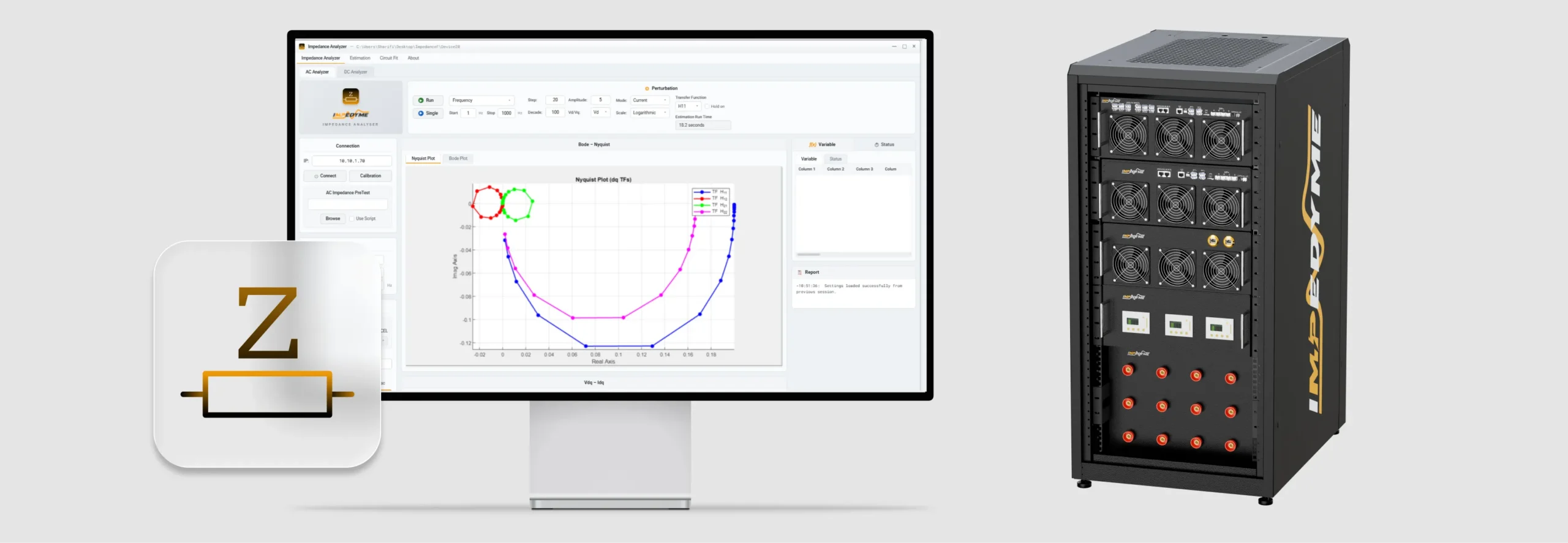
Impedance Analyzer
An impedance analyzer measures how a component, material, or entire power system opposes alternating current across a range of frequencies. Where a multimeter gives you a single DC resistance and an LCR meter gives you a value at one fixed frequency, an impedance analyzer sweeps frequency and returns the full complex impedance — magnitude and phase, or resistance and reactance — at every point, then plots it as a curve you can interpret.
That curve is where the engineering value lives. It reveals self-resonant frequencies, hidden parasitics, battery state of health, and — critically for modern power electronics — whether a grid-connected converter will stay stable when it meets a real grid. This guide explains what an impedance analyzer measures, the physics behind it, how to read Bode and Nyquist plots, how dq-frame impedance analysis works for three-phase systems, and what to look for when selecting one.
What Is an Impedance Analyzer?
An impedance analyzer is test equipment that measures complex electrical impedance as a function of test frequency. Impedance is the alternating-current generalization of resistance. In a DC circuit, the opposition to current flow is simply resistance. Under AC excitation, voltage and current are usually shifted in time relative to each other, so the opposition to current flow has two parts:
- Resistance — the real, energy-dissipating part, which turns electrical energy into heat.
- Reactance — the imaginary, energy-storing part, which shuttles energy in and out of electric and magnetic fields.
Reactance itself depends on frequency. Inductive reactance grows as frequency rises, while capacitive reactance shrinks as frequency rises. Because reactance changes with frequency, every real component and system traces a characteristic impedance curve as frequency is swept — and capturing that curve is exactly what the instrument does.
Impedance can be described two equivalent ways: as resistance plus reactance, or as a magnitude paired with a phase angle. The magnitude tells you how much the device opposes current; the phase angle tells you what kind of opposition it is — purely resistive, partly capacitive, or partly inductive. The inverse view of impedance is admittance, which describes how easily current flows rather than how strongly it is opposed, and is sometimes the more natural way to describe a device.
Impedance Analyzer vs. LCR Meter vs. Multimeter
These three instruments are often confused. The difference is what they measure and how much of the picture they show.
| Instrument | What it measures | Frequency behavior | Best for |
|---|---|---|---|
| Multimeter | DC voltage, current, resistance | DC only — no reactance | Quick checks, continuity, DC values |
| LCR meter | Inductance, capacitance, resistance (plus Q, D, ESR) | One fixed frequency or a few | Fast production pass/fail |
| Impedance analyzer | Full complex impedance: magnitude, phase, resistance, reactance | Sweeps a frequency range | Characterization, EIS, stability analysis |
The Measurement Principle: Perturb, Measure, Compare
Every impedance measurement — no matter the hardware — is the same experiment repeated at many frequencies:
Apply
A controlled small-signal AC perturbation — a voltage or current stimulus — to the device under test.
Measure
Both the voltage across the device and the current through it — keeping track of their timing relative to each other.
Compare
The two signals, preserving the phase relationship, to obtain the complex impedance at that frequency.
Sweep
Step the frequency and repeat — building the full impedance spectrum, point by point.
The four settings engineers control most
Modern digital analyzers — including Impedyme's — sample voltage and current over time and use frequency-domain processing to recover magnitude and phase at each excitation frequency. Faster than lock-in detection, and able to stimulate many frequencies at once.
Frequency Range
Start and stop frequencies of the sweep.
Sweep type
Logarithmic (points per decade) or linear (zoom a band).
Resolution
Points per decade, or total number of points.
AC Ampltude & DC Bias
Perturbation level and the device's operating point.
Reading the Results: Bode and Nyquist Plots
Impedance spectra are presented two main ways. Knowing how to read both is the core skill.
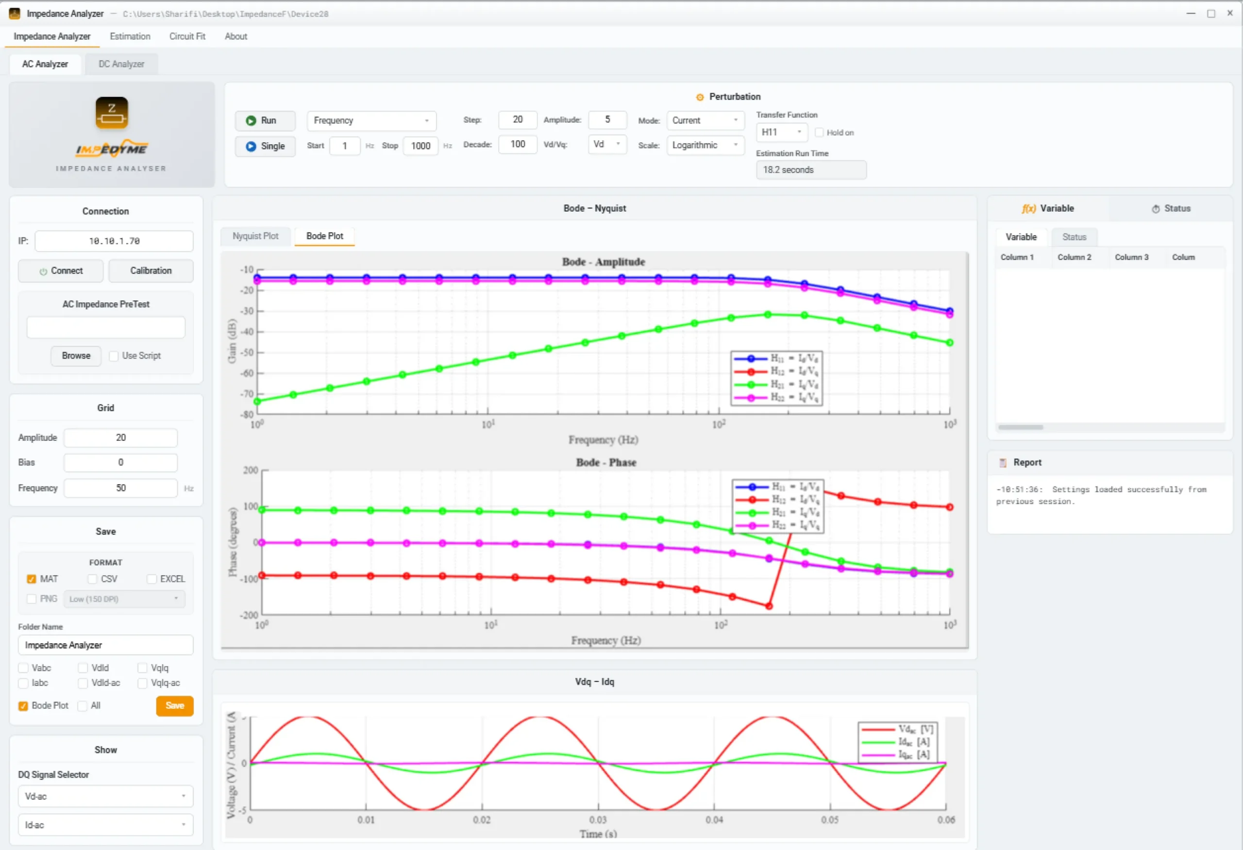
Two stacked graphs against a log-frequency axis.
Magnitude in ohms or decibels; phase in degrees. Bode plots make frequency explicit — read off value and phase at any frequency, spot corner frequencies, and see where a device transitions between resistive, capacitive, and inductive behavior.
Resistor
Flat magnitude, zero phase.
Capacitor
Magnitude falls as frequency rises; phase near −90°.
Inductor
The Nyquist Plot
A Nyquist plot maps the imaginary part of impedance against the real part on a single plane, with frequency as an implicit parameter that moves you along the curve. Both axes must use the same scale, because every point represents one complex impedance value.
Nyquist plots are the standard in electrochemistry and stability analysis because their geometry maps directly onto physical processes:
- A semicircle corresponds to a parallel resistor–capacitor process.
- The high-frequency intercept on the real axis gives the ohmic or series resistance.
- The diameter of a semicircle equals the charge-transfer (or polarization) resistance.
- A 45-degree straight tail at low frequency is the Warburg response — the signature of diffusion-limited transport.
- Multiple semicircles mean multiple processes with different time constants.
Sweep Parameters That Shape the Curve
1
Fusion of real‑time emulation and EIS
2
Automation and openness
3
Tight hardware integration
Impedance Analyzer vs. Vector Network Analyzer
Impedance Analyzer
Direct measurement, widest impedance range
An impedance analyzer determines impedance directly from the measured voltage and current. It is strongest from very low frequencies up into the low-gigahertz range, delivering high absolute accuracy across an extremely wide impedance range — from milliohms to many megohms and beyond.
Best for:
- Component and material characterization
- Electrochemical impedance spectroscopy
- Power-electronics work from DC to megahertz (and into the low gigahertz)
Vector Network Analyzer
Reflection-based, optimized for RF matching
A vector network analyzer measures how much of a signal reflects from the device and converts that into impedance. It dominates at high RF and microwave frequencies, but reaches its best accuracy only when the device under test is near the standard fifty-ohm system impedance — accuracy degrades for very high or very low impedances.
Best for:
- Antennas
- Filters
- Transmission-line work where high-frequency matching matters
Applications of the Impedance Analyzer

Grid-connected inverters

DC-DC & motor drives

Battery impedance / EIS

Fuel cells & electrolyzers

Passive components

PCS, EV charging, data-center
Calibration and Accuracy
A raw measurement includes the cables, not just the device.
Calibration removes the parasitics of cables, fixtures, and connectors by measuring reference standards. It must be performed at the device connection plane, and re-run whenever the frequency range, fixturing, or cabling changes.
For low-impedance work, four-terminal (Kelvin) connections are essential — they separate current-forcing and voltage-sensing paths, removing lead resistance and inductance. Poor calibration is one of the most common causes of unstable or biased readings.
The Impedyme Impedance Analyzer
AC dq-matrix measurement
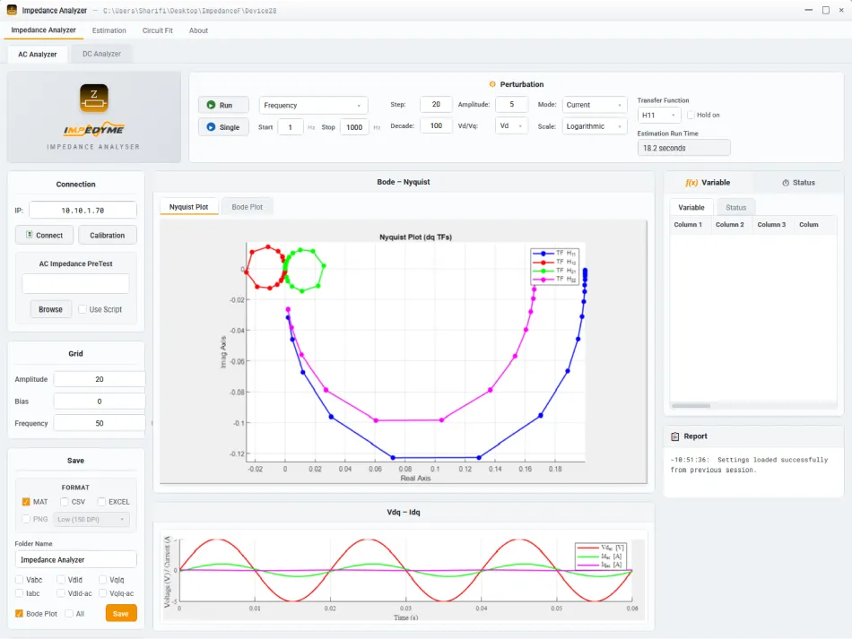
Measures the full two-by-two dq transfer-function set — H11 through H22 — of a three-phase system. Bode, Nyquist, and time-domain DQ signals let you verify the perturbation and assess converter–grid stability before it reaches the field.
Frequency sweep and injection
Start and stop frequency in hertz with step, decade, and points-per-decade settings on logarithmic or linear scale. Selectable current or voltage perturbation with adjustable AC amplitude and DC bias keeps the device at its operating point during measurement.
Connectivity and protection
Connects over Ethernet with a built-in Calibration function and a Use Script automation option. Configurable voltage, current, temperature, and AC-amplitude limits keep the device under test safe throughout the sweep.
DC battery impedance and EIS
Battery impedance testing with a Battery Impedance PreTest, measuring per-terminal impedance (Terminal A, B, C) with Nyquist and Bode displays. Three-phase voltage and current signals per phase support EIS-style diagnostics for state of health and internal resistance.
Transfer function and axis selection
Direct selection of H11 through H22 and the direct- or quadrature-axis perturbation to apply — matching the core requirement for two independent injections in dq impedance measurement, with each one under explicit control.
Export and reporting
Results export to MAT, CSV, Excel, and PNG — including three-phase voltage and current, direct- and quadrature-axis signals, and full Bode and Nyquist data ready for reports or further analysis.
dq-Frame Impedance Analysis for Three-Phase Power Systems
Three-phase AC quantities are constantly changing sinusoids, which makes direct impedance analysis awkward. The Park transformation solves this by projecting three-phase signals onto a reference frame that rotates with the grid fundamental, synchronized through a phase-locked loop (PLL). In this rotating dq frame, balanced steady-state quantities become steady values, the problem collapses to two axes — direct and quadrature — and the same Nyquist-based stability tools used for DC systems apply. Because the two axes are coupled, a three-phase port is described not by a single impedance but by a two-by-two matrix, measured in Impedyme's Impedance Analyzer as four transfer functions: H11 and H22 for the direct- and quadrature-axis responses, and H12 and H21 for the cross-coupling between them. The direct-axis channel reflects the current loop and filter dynamics, while the quadrature-axis channel is shaped by the PLL and can act as a negative resistance over its bandwidth — a key destabilizing mechanism in weak grids.
This matters because a grid-connected converter and the grid form a source–load pair whose stability depends on how their impedances compare across frequency. When a converter's negative-resistance region overlaps a network resonance — such as a series-compensated line — the result can be sub-synchronous oscillations or harmonic instability, interactions that have caused real-world damage to converters and series capacitors. These instabilities have no fixed frequency; they shift with grid strength, compensation level, and control tuning, which is exactly why measured, frequency-resolved dq impedance is needed rather than a model alone. Resolving the full matrix requires two independent perturbations — one predominantly on the direct axis, one on the quadrature axis — in either voltage or current mode; the recorded three-phase signals are transformed into the rotating frame and processed in the frequency domain to extract magnitude and phase at each point.
Built on a Real-Time PHIL/HIL Platform
The real differentiator is the validation platform behind the application. Impedyme's Impedance Analyzer runs within PowerHIL Studio on the CHP Series — a modular, FPGA-powered Combined HIL and Power-HIL (PHIL) testbench. The CHP Series resolves simulation time steps on the order of tens of nanoseconds on AMD/Xilinx Zynq UltraScale+ MPSoC fabric, fast enough to capture rapid converter dynamics while spanning slower grid behavior. Companion tools — GridSim Studio, BatterySim Studio, MotorSim Studio, DroneSim Studio, FPGA Scope, Charger Box, and HIL/RCP-Box — extend the ecosystem across grid, battery, motor, and drone validation.
Frequently Asked Questions
Make Impedance Analysis More Powerful
Explore a complete impedance analyzer platform for dq stability assessment, battery EIS, and converter–grid validation.


