Solar inverter test

The DC Side of a Solar Inverter Test: PV Source Emulation and MPPT Performance

Every credible solar pv inverter test begins with the source. If the DC source does not behave like a real array, everything measured downstream is suspect.

Understanding PV Array Characteristics: The Prerequisite to PV Inverter Testing

A photovoltaic array is neither an ideal current source nor an ideal voltage source. It is a nonlinear device whose delivered current depends on the voltage the connected load imposes on it. Three physical relationships drive everything that follows in a pv inverter test:

• Short-circuit current is governed almost entirely by irradiance. More sunlight yields proportionally more available current. When a cloud edge passes, current drops almost instantaneously.
• Open-circuit voltage is governed by cell temperature. The array’s voltage ceiling rises as modules get colder and falls as they heat up. Irradiance affects it only slightly. This is why cold, bright mornings produce the highest string voltages of the year.
• Effective source impedance changes continuously along the curve. Near the short-circuit end the array behaves like a current source, holding nearly constant current across a wide voltage span. Near the open-circuit end it behaves like a voltage source, where a small change in current swings the voltage dramatically. Every operating point corresponds to a different effective impedance.

Between those extremes sits the maximum power point — the single “knee” where current and voltage together yield the most power. It moves continuously as irradiance and temperature change, and the inverter’s tracker has to follow it. Reproduce that movement faithfully and your solar inverter testing results mean something. Fail to, and they do not.

Why Solar PV Inverter Testing Is Fundamentally About PV Emulation

Here is the shift in perspective that governs the whole DC side of pv inverter testing.

In practice, inverters are almost never validated as isolated devices. What matters is how the inverter behaves when coupled to a realistic PV source under changing environmental and grid conditions. The core of a solar inverter test is not only power conversion efficiency or control stability — it is how the inverter interacts with a dynamic, nonlinear PV input.

That raises an obvious problem. Real panels cannot serve as a controlled test source, because the variables you would need to control are precisely the ones you cannot: irradiance, cell temperature, shading. A test you cannot repeat is not a test. The conclusion is unavoidable: meaningful validation requires programmable PV emulation.

Why a Generic DC Power Supply Is Not Sufficient for PV Inverter Testing

Engineers new to this application often reach for a laboratory programmable DC supply. It does not work, for four specific reasons:

• It is not equivalent to a PV source. A conventional supply has a hard output characteristic — it holds the programmed voltage regardless of current draw, presenting very low output impedance. A real array presents a curved, operating-point-dependent impedance.
• It cannot reproduce I–V dynamics. No curvature, no defined maximum power point, no response to simulated irradiance or temperature change.
• It breaks the closed-loop MPPT interaction. This is the critical failure. MPPT algorithms deliberately perturb the operating point and observe the resulting power change. A stiff voltage source regulates that perturbation away, so the tracker is never honestly exercised. The measurement you get back is meaningless.
• It cannot reproduce PV-side faults. A generic supply regulates voltage, current and power. It cannot produce partial shading, multi-knee curves, string mismatch or abrupt array-side dropouts.

The practical consequence is that a solar inverter test run against a generic supply will report a tracking efficiency the device will never achieve in the field — and will report it with confidence.

Hardware Foundation of Solar Emulation: What a PV Simulator Must Do

From a hardware perspective, PV simulation is a control problem executed by power electronics. The power stage must respond quickly and predictably so that the intended array model is expressed at the terminals the inverter actually sees. Five requirements separate a genuine simulator from a supply with a curve-shaped setpoint:

Fast and predictable voltage and current dynamics. Real irradiance changes abruptly during cloud transients, and the inverter perturbs its own operating point continuously. The simulator must let terminal voltage and current move along the I–V curve at a realistic rate. Slew rate and control bandwidth determine whether start-up, curtailment and ride-through recovery behaviour are trustworthy.

Low output capacitance and limited electrical interaction. A real array holds very little stored energy, so its operating point can move almost instantly. A simulator with excessive output capacitance smooths the I–V transitions and flatters the inverter’s measured tracking efficiency — the device under test effectively sees a laboratory capacitor bank rather than a solar array. Two labs running the same solar pv inverter testing protocol on differently damped simulators will report different numbers for the same product.

Regenerative capability. When the inverter pushes energy back toward the source, a non-regenerative simulator can see its output voltage overshoot, risking a protective shutdown or component damage. A source-and-sink architecture absorbs it.

High curve resolution and dynamic profiles. Faithful representation of multi-knee shading curves requires many I–V points with smooth interpolation between them. Irradiance and temperature need to be treatable as time-varying inputs — ramps, steps, oscillations, recorded weather traces — with the curve reshaping continuously.

Scalable power through reliable parallel operation. A microinverter programme and a multi-megawatt central inverter programme are the same test problem at different scale. Parallel operation must not degrade dynamic performance.

Solar PV Inverter Test on the DC Side — What Good Looks Like

MPPT efficiency is the headline DC-side metric of any solar inverter test, and it splits in two.

Static MPPT efficiency holds irradiance constant on a fixed I–V curve and measures how tightly the tracker settles on the peak. It is evaluated across a range of power levels — typically from a few percent of rated up to full rated — and at low, medium and high MPP voltage. It exposes steady-state oscillation around the peak and any voltage-dependent bias in the algorithm.

Dynamic MPPT efficiency ramps irradiance up and down on defined gradients with defined dwell times, forcing the tracker to chase a moving target. Prescribed ramp rates span from very slow to very fast. A tracker that perturbs too cautiously lags a rising ramp; one that perturbs too aggressively wanders off-peak. The score is how much of the available energy was captured during the transitions.

The European standard EN 50530 defines this static-and-dynamic split and is the most widely used reference; IEC 62891 covers the same ground in the IEC framework, with steady-state conversion efficiency measured per IEC 61683. Overall efficiency is the product of conversion efficiency and static tracking efficiency, with dynamic tracking reported separately. Regionally weighted single-number efficiencies — the California and European weighted figures — combine efficiency at several load points using climate-representative weights.

It is worth being blunt about why this matters commercially. Modern inverters commonly convert at around 98% but track at 96–97%. An inverter that converts at 98% and tracks at 96% is a 94% device in the field. Over a 25-year asset life, a single percentage point of tracking deficit is measured in megawatt-hours per megawatt installed.

One structural gap worth knowing: the standardised MPPT efficiency procedures do not cover shaded curves with multiple local maxima. Global-peak-search behaviour under partial shading is real, commercially significant, and outside the scope of the standard test — which means it has to be included in your pv inverter testing plan deliberately, or it will not be tested at all.

The AC Side of PV Inverter Testing: Grid-Code Compliance and Power Quality

This is where most published content on solar inverter testing stops, and where the harder engineering begins.

Anti-islanding. If the utility supply is lost, the inverter must detect that it is energising an island and cease to energise within the required window — under the prevailing North American interconnection standard, within two seconds of island formation. The test is deliberately adversarial: a resonant load is tuned to match the inverter’s output so precisely that utility removal produces almost no detectable change in voltage or frequency. Islanding tests are typically run at multiple output levels, commonly around one-third, two-thirds and full rated power.

Voltage and frequency ride-through. The inverter must remain connected through disturbances it should survive. Ride-through requirements are organised into performance categories, with defined voltage bands and clearing times — for example, a high-voltage threshold cleared in a fraction of a second, and lower-magnitude excursions tolerated for a couple of seconds.

Grid-support functions. Volt-var control adjusts reactive power output along a piecewise curve defined by voltage breakpoints. Volt-watt curtails active power at high voltage. Frequency-watt provides droop response to frequency deviation. Constant power factor and constant reactive power modes are also specified. Which functions are enabled, and with what settings, is typically the utility’s decision.

Power quality. Harmonic distortion is limited — the common North American ceiling is 5% total demand distortion at rated output. DC current injection is limited because it saturates distribution transformers, with limits and test methods defined in the inverter safety standard. Flicker must remain imperceptible.

Ramp, start-up and reconnect. Start-up power ramp rate is controlled. After a trip, the inverter must observe healthy voltage and frequency for a defined period — commonly five minutes — before reconnecting, with a randomised delay so that a feeder full of inverters does not all reconnect simultaneously.

Reactive power capability and priority. Different performance categories require different reactive ranges, and during a disturbance the inverter must prioritise either active or reactive current according to its configuration.

Several of these behaviours are difficult or unsafe to reproduce on a conventional physical bench. We return to that in the validation-gap section below.

Solar PV Inverter Test Procedures: What Each Test Actually Measures

Ask ten engineers to list the tests in a solar pv inverter test programme and you will get ten different lists. The confusion is avoidable, because the governing conformance standard already sorts every test into one of four classes — and the class tells you who runs it, how often, and what it proves.

Type tests are where design risk lives, so that is where the rest of this section concentrates.

The most complete published inventory of what a thorough pv inverter testing campaign actually exercises comes from utility and national-laboratory dynamic test procedures. These are worth studying closely for one reason: they are characterisation methods. They record how the device behaves rather than issuing a pass or fail. That makes them a far better template for internal validation than a conformance checklist, because the output is a behavioural profile you can compare across firmware revisions rather than a single binary result.

Test Bench Setup and Instrumentation

The bench is consistent across every test below: a grid simulator capable of injecting realistic voltage and frequency deviations, a PV simulator emulating array behaviour, the inverter under test, a variable load bank with real and reactive elements, a power analyser, and a control computer running the sequence. Wiring differs between split-phase and three-phase configurations.

Measurement discipline matters more than most benches allow for. Voltage and current are captured on both the inverter side and the grid side, time-synchronised, at sample rates chosen per test. Real power, reactive power, frequency and harmonic content are then derived from the raw waveforms — not read off summary meters. This distinction is not academic. A summary meter reports what happened over a window; a synchronised waveform capture shows you the sub-cycle sequence of events, which is the only way to distinguish “the inverter tripped because of the sag” from “the inverter tripped 40 milliseconds after the sag recovered.”

Safety infrastructure covers protection breakers and fuses on both the DC source-to-input path and the AC source-to-output path. Grid simulators typically add internal input and output breakers, a contactor and layered protection. Standard electrical PPE and lockout practice apply throughout — several of the tests below deliberately create conditions the inverter is designed to escape from.

DC-Side Solar Inverter Test Procedures

Three tests, all concerned with how the inverter behaves when its energy source appears, disappears or moves:

• DC “on” time delay. With the grid simulator already at steady state, the PV simulator output is switched on. The measurement is how long the inverter takes to begin generating AC and how quickly it ramps to nominal. Repeated runs matter here — inconsistent start-up timing across identical trials usually points to a race condition in the start-up state machine, and it will not show up in a single run.
• DC “off” delay. With the inverter generating, the DC connection is opened. The measurement is time to reach minimum current output. This is a safety-relevant number: it bounds how long the AC terminals remain live after the array is disconnected.
• Irradiance profile response. A recorded or synthesised irradiance profile is played into the PV simulator. This captures transient and aggregate response to rapid shading — and it is the test where MPPT algorithms most often reveal that they hunt, stall, or fail to reacquire the peak after a deep cloud transient.

AC-Side Solar PV Inverter Test Procedures

Thirteen tests, each injecting a specific grid disturbance while the analyser records the response. The value is not the list — it is knowing what each one is looking for.

Conservation voltage reduction is the test most often skipped and least often understood. Utilities lower feeder voltage during peak periods to reduce customer demand. An inverter running autonomous volt-var support is, by design, trying to hold voltage up — the two objectives are directly opposed. Utility-scale analysis has found the interaction is often inconsequential in practice because CVR events tend to coincide with low PV output, but “often” is not “always,” and it is a behaviour worth characterising rather than assuming.

Short-circuit contribution is not a nuisance measurement. Protection engineers need a defensible number for fault-current contribution, and inverter fault behaviour is nothing like a synchronous machine’s — it is defined by current limiting in firmware, not by machine physics. Work on three-phase PV inverters has measured fault-current contribution reaching roughly twice nominal peak current, with the exact figure depending entirely on the control implementation.

Three-Phase Unbalance Tests

Two additional tests apply to three-phase units: unbalanced under-voltage transients and unbalanced over-voltage transients.

Unbalance deserves disproportionate attention because it breaks assumptions that balanced testing quietly validates. Research on three-phase PV inverters under unbalanced conditions has found that volt-var reactive control responds to the positive-sequence voltage rather than the measured phase voltages — so the control acts on a quantity the test engineer may not be monitoring. The same work found the frequency-support activation point shifted measurably under unbalance: still inside the grid-code window, but not where a balanced-condition test would have predicted. If your test matrix is balanced-only, you have validated a subset of the real operating envelope.

Advanced Grid-Support Function Tests

Six tests covering the functions a modern certificate actually claims:

• Start-up power ramp rate — controlled ramp on entering service
• Voltage ride-through — remaining connected through disturbances the inverter should survive
• Over-frequency power curtailment — droop reduction of active power above nominal frequency
• Autonomous power factor adjustment — reactive output following the configured power factor mode
• Autonomous voltage support, under-voltage — reactive injection to raise local voltage
• Autonomous voltage support, over-voltage — reactive absorption to lower it

These are the tests where certificate claims and field behaviour most often diverge, because they are the most configurable. A volt-var curve is a set of numbers in a settings file, and a firmware update can change how those numbers are interpreted without changing the numbers themselves.

Where Simulation Changes the Economics of These Tests

Several of these procedures are expensive precisely because of what they require physically. Anti-islanding is the clearest example: the traditional method uses a bank of physical resistive, inductive and capacitive elements tuned to resonance at nominal frequency. Those banks are large, costly and generate substantial heat, and re-tuning them for each test point consumes hours.

Published work has demonstrated the same test executed with a virtual RLC load inside a real-time simulation, with the inverter interfaced through a power amplifier. The device under test cannot distinguish the simulated load from a physical one, but the load becomes a software parameter — which means the test point sweep that took days becomes an automated overnight run.

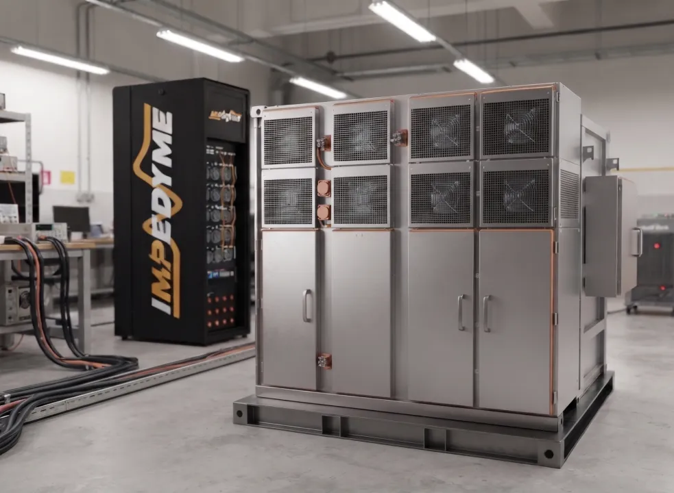
The same logic applies across the AC-side list. Voltage and frequency ramps, oscillations, unbalance and short circuits are all disturbance definitions, and a real-time simulated grid produces them on demand at full power. Impedyme’s PHIL platform runs this entire disturbance library at megawatt scale through GridSim Studio, with programmable grid impedance so that each test can be repeated at different short-circuit ratios — turning a one-dimensional pass/fail into a two-dimensional stability map.

PV Inverter Performance Test Criteria: Producing Numbers You Can Defend

The procedures above characterise dynamic behaviour. A separate body of protocol work answers a different question entirely: how do you run a pv inverter test that produces performance numbers meaning the same thing in two different laboratories?

This matters commercially. Datasheet efficiency figures are compared across vendors, written into yield models, and used to size assets. If two labs measure the same inverter differently, every downstream number is contaminated. The protocol answer comes down to three things: control the conditions, bound the measurement error, and report what you actually did.

Establishing Valid Conditions for Solar Inverter Testing

Thermal stability must be defined, not assumed. A canonical definition: three successive readings taken at least thirty minutes apart, following an extended run-in period, varying by no more than one degree. Efficiency measured on a cold inverter is not efficiency; it is a best case that no field installation will ever see.

Measurement uncertainty is bounded explicitly. True-RMS measurement is mandatory — average-responding instruments misread distorted waveforms, which is exactly the condition you are trying to quantify. Allowable uncertainty on voltage, current and power is held tight, with frequency and temperature accuracy specified separately. AC ripple riding on the DC lines must be accounted for whenever it becomes significant relative to the DC magnitude, because ripple that the analyser attributes to DC input power inflates the denominator and understates efficiency.

The source requirements contain the most revealing detail in the whole protocol. The DC supply must have low output ripple, capability exceeding the inverter’s rated input, and adjustability across the full input voltage range. It may also require external series impedance — so that the supply and the inverter do not fight each other for control of the operating point.

Read that again, because it is the entire argument for PV emulation stated by a performance protocol that predates modern simulators. Even a laboratory DC bench has to be deliberately softened to behave in a PV-like manner, or the solar inverter test result is invalid. A programmable PV simulator does this by design rather than by adding series resistors.

The Core Measurements in a Solar PV Inverter Test

Eight measurements carry the weight of the entire performance programme.

DC input characterisation. Two numbers: the maximum power point voltage tracking range and the maximum power point current tracking range. These define the windows over which the inverter will actually hold the MPP — which is not the same as the input ranges printed on the datasheet, and the gap between the two is where early-morning and late-afternoon yield disappears.

Maximum continuous output power. Sustained deliverable power under defined thermal conditions. The word doing the work is continuous.

Conversion efficiency. Usable AC output relative to total input, reported across load points rather than as a single peak figure. Peak efficiency is a marketing number; the efficiency curve is an engineering one.

Maximum power point tracking accuracy. A steady-state response test and a dynamic response test, reported as array utilisation — the fraction of available energy the inverter actually extracted. Any value below unity is the direct, quantified cost of imperfect tracking, and it compounds every day for twenty-five years.

Tare losses. Standby and self-consumption levels, plus the input power thresholds at which the unit wakes up in the morning and shuts down at night. Tare is a small number that runs for a long time: it is drawn from the grid every night for the life of the asset, and a high shutdown threshold means the inverter sits idle through low-irradiance periods that a lower-threshold unit would harvest.

Power foldback. Two distinct derating behaviours that pv inverter testing frequently conflates:

• Foldback with temperature — the inverter shifts its operating point to a reduced power level once monitored component temperatures reach their limit, protecting the semiconductors, and returns to the optimum point as it cools.
• Foldback with high array output — deliberate limiting when the array delivers more than the inverter’s AC rating, common in the deliberately oversized DC-to-AC ratios now standard in utility-scale design.

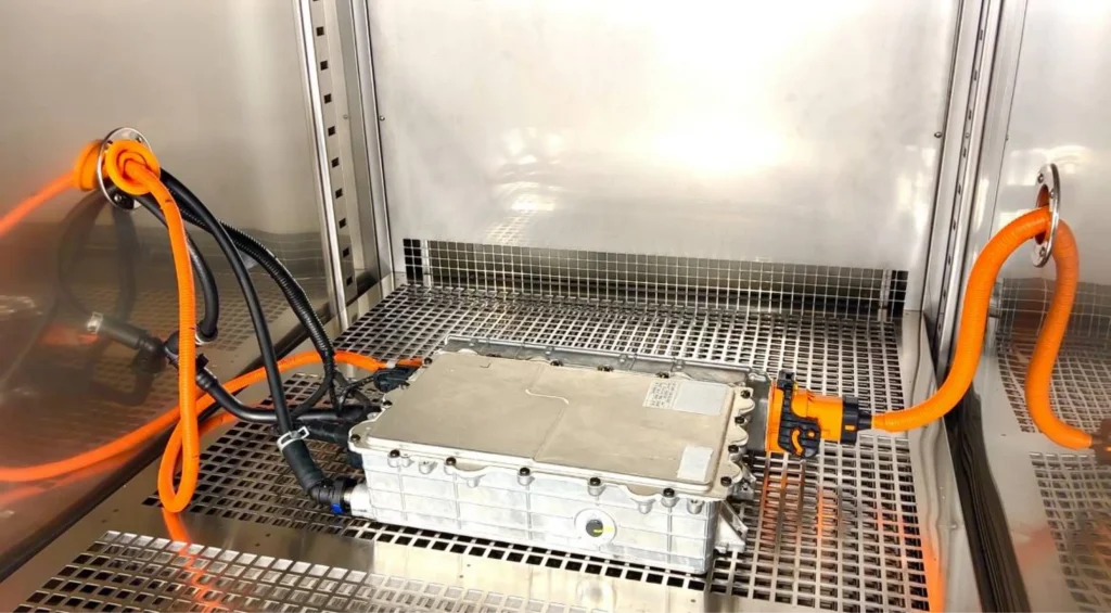
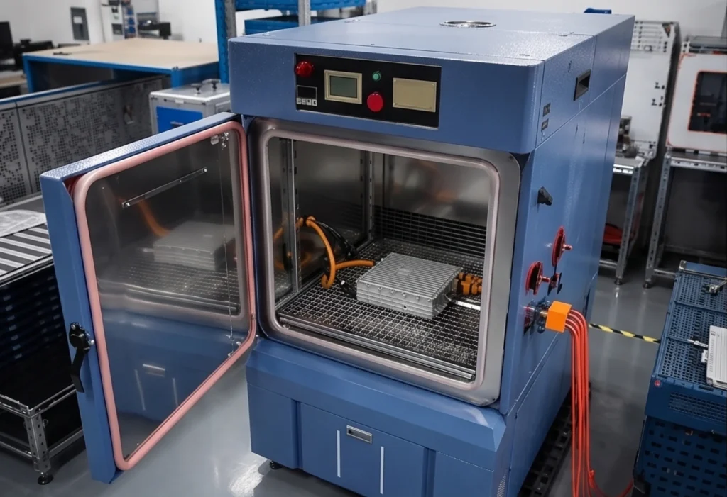
Temperature derating is worth flagging as a genuine gap in the standards landscape: no international standard governs this characteristic test, so methods are manufacturer-defined and typically require a thermal chamber. Comparative laboratory work has found measurable discrepancies between manufacturer-published derating curves and experimentally derived ones — which means the derating behaviour written into your yield model may not be the behaviour the hardware exhibits.

Inverter performance factor and inverter yield. The roll-up. This is the metric that predicts field energy production, and the number an asset owner actually cares about — every measurement in this solar pv inverter testing sequence exists to make this one credible.